Opmmur
Time Travel Professor
- Messages
- 5,049
I have been a Ham Radio Operator for many years. You can use the same
type of set up for a radio Antenna also.
HOW DOES AN EARTH DIPOLE WORK?
By Renato Romero
Although in internet many materials can be found about earth dipoles used as antennas, to understand how they works can be very complicated. With what principle does it work? What is the frequency range where it can be used with good profit? What about reception diagram? What's the signal component received with an earth dipole: electric field or magnetic filed? With what polarization?
And still: why some signals present on air (as Schumann resonaces) can't be received with earth probes? And why some signals received with earth dipole are not receivable on air? In this article we will search some answer to these questions.
DEFINITIONS AND APPLICATIONS
With "earth dipole" we meana reception system composed by two earth connections, spaced each other by some tens meters, used as receiving or transmitting antenna. They are used in different applications, professional, military and for hobby:
- as transmitting antenna for 82 Hz and 76 Hz signals, directed to the submarine in immersion (during missions)
- for earthquake radio precursors monitoring, see the ELFRAD group activity
- by some radioamators for the 137 kHz band reception
- by some SWL for medium wave and long wave broadcast monitoring
- by geologist for geophysical prospecting and underground tomography
- from the archeologists, for ruins location finding
In this script we will limit our study to the earth dipole used as receiving antenna below 22 kHz.
SOME RECEPTIONS COMPARISON
A first wide band test shows very similar results obtained using an earth dipole compared to a stylus reception.
 VLF Range
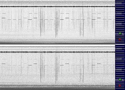
The picture beside shows some seconds of nighttime reception in a 1 Hz to 22 kHz frequency range.
The above part has been received with an 7m vertical stylus, placed 50m from my home in the garden, far from electric lines. Alpha signals, RTTY and statics are clear. Below 2 kHz some hum noise.
Part below shows the same signal received with a 25m earth dipole, E-W oriented, and installed in the same place of the stylus. Signals are very similar. Hum noise is a little stronger than before but substantially two pictures show the same signals.
But going down in frequency some differences begin to appear:
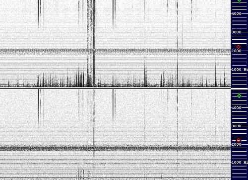 VF (Voice Frequency) Range
In the part above (received with stylus) many long distance statics (the ones below 1 kHz) appear in the spectrogram. They extend their components down to few Hz.
But in the part below (coming from earth dipole) they seem to become more and more weak going down in frequency. The long distance statics have almost disappeared under the 500 Hz.
Reception landscape appears clear and complete in the next spectrograms:
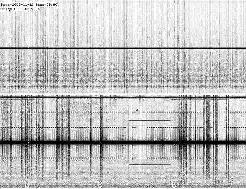 ELF/ULF Range
Where it is shown a comparison between the two different reception system in the frequency range from 0 to 100 Hz. Here differences appeared light in the voice frequency range (300 Hz - 3 kHz) become substantial.
In the part above we can see Schumann resonaces, 50 Hz hum noise tone and some statics.
In the part below 50 Hz tone appears stronger (with a 100 Hz tone, invisible with stylus reception), different wide band bursts are present, many tones mirrored to 50 Hz signal, an hiss below 15 Hz and no evidence of Schumann Resonances.
How to explain this marked difference of behavior in the different ranges of frequency?
SOIL IMPEDANCE MEASUREMENTS
Some preceding experiences demonstrate me that an earth dipole is not so easy to understand. Following the intention to discover how it receives signals present on air, I decided to measure the impedance of the soil, seen by two earth probe 55m meters far each other.
 First tentative was with a bridge measuring instrument: an ESI 250. It can measure very low inductance value, also with Q factor very low, below 1, injecting a low sinusoidal current of 1 kHz.
But results by measurements were too strange: sometimes I saw between the two stakes an inductance of 50 mH (an incredible value, too high), and sometimes the same measure repeated 30 minutes later gave values of 20 or 30 mH.
And even more strange: changing the dipole direction the inductance value changes. A spectrogram analysis of the signal used by bridge for its null gave me the answer.
The reason was in the ground: the 50 Hz hum noise with all harmonics components falses the measures, and the bridge finds its null not on his real signal but on the 50 Hz 20th harmonics: the 1000 Hz coming from electric line. It changes in level in the time and change in direction with the dipole: values change consequently.
Table of tests is not reported here, because results are with any meaning.
After a short consultation with Wolfgang (DL4YHF) I decided to change this measurements system.
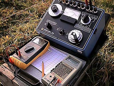
 Picture beside shows the new measurement setup, composed by 2 channels digital oscilloscope, a signal generator and a 1 kOhm resistor.
Signal generator injects its current in the ground by earth probe, passing through the 1 kOhm resistance. First channel of oscilloscope reads voltage on the 1 kOhm resistor (V2-3), second channel on the earth dipole (V1-3). Tests were made at different frequencies, starting from 50 Hz to 100 kHz. For every frequency was recorded the two voltage values and the delta time from the two signals (Dt).
Both the instruments (signal generator and digital oscilloscope) where battery maintained, to avoid ground loops and have floating measurements points done.
All data were tabulated in an excel table (first 5 columns). The other 8 columns were used with mathematical formulas to calculate values for every frequency of:
Idipole
Z
Phase
Xc or XL
R
Q
C or L =
=
=
=
=
=
= Current in the earth dipole
Impedance module of the earth dipole
Grade and radiant between voltage and current in the earth dipole
Reactive component of impedance
Active component of the impedance
Q factor
Value of the reactive component in the ground
Here below the results:
Results was for me a surprise: current was not in late but in advance respect the applied voltage. The graph shows clearly the results:
 Looking into the earth stakes we don't see an inductance: we see a capacitance!
Light blue curve shows this phenomenon. And capacitance value grows going down in frequencies. At 50 Hz we can observe a big value of 60 uF. Here a reason because the virtual underground loop can not work below 2 kHz: weak inductance value can be nulled by this underground capacitance.
We can also observe an increasing of the capacitive reactance going up in frequency and a decreasing of the resistive values at higher frequencies.
But how can be possible an underground capacitance if current paths describes a loop? Where is the origin of this new component?
FREQUENCY DEPENDENT RESISTIVITY AND INDUCED POLARIZATION
A complete explanation of this phenomenon can be found in a document of University of California of BERKELEY, where the "induced polarization" phenomenon (this is the correct name) is explained. This document observes that the measured resistivity of a soil is function of the frequency in the range from 0.1 mHz to 10 kHz, and that voltage and current are not in phase especially if soil contains clay (like in my measures).
 Picture (taken from that site) shows the real component where current is in phase with applied voltage (resistance) and the imaginary component where the current is 90 degrees out of phase, in squared (capacitance). Here, as in the graph above we can see that the resistivity decreases with increasing frequency, and that the imaginary component with his maximum at fr: the relaxation frequency. The range where we can see the maximum change of resistivity and where imaginary component maximizes is called dispersive region.
Soil electrical response suggests an energy storage mechanism like in a capacitor. Then, the equivalent circuit of the soil can be synthesized as the following circuit:
 At DC the capacitor is an open circuit and all the current passes through the sum of R1 and R2, developing a voltage Vp = I (R1 + R2). As the frequency increases, current can flow through the capacitor, which decreases the overall resistance. Finally at high frequency the current is effectively short circuited by the capacitor and the voltage developed is simply I R1.
Between the DC and high frequency limits, the voltage across the capacitor is phase shifted 90° from the current and so adds an imaginary component to the total voltage measured across the circuit, which peaks midway between the low and high frequency asymptotes. Thus, we see that this circuit faithfully reproduces the key features observed in the measurement
Capacitance is basically a ionic separation under the application of an electric field of free charges, ions, that move through the fluid. How can we imagine then, an earth dipole as receiving antenna? The following models try to give a possible explanation.
THE UNDERGROUND LOOP MODEL
The first model easy to think corresponds to an underground loop. Following the current paths through the earth (includes by two earth probe with a DC voltage applied), we can observe an underground current loop. Loop model can also explain why sensitivity decreases at low frequency, as we can see in the ELF/ULF spectrogram above.
 Virtual Loop dimensions are similar to a square loop. Then, for a 25m earth dipole we can suppose an underground virtual square loop of 25m x 4 = 100m.
DC resistance really measured by the two stakes was about 500 Ohm. Using a software simulation of G4FGQ (rjeloop3.exe) we can calculate the loop inductance and the wire equivalent diameter. For a 25m earth dipole of the picture, estimated inductance is 0.26 mH and the equivalent loop results composed by a wire of 0.06 mm diameter (more little than a hair).
(A fast loop test made by one square turn 25m side horizontally placed was measured, obtaining 0.29 mH. Then the 0.26 mH value above can be considered valid)
Using the formula
F = XL / (2 x 3.14 x L)
we can calculate the low frequency corner, where the underground loop stops being an antenna, and the resistance effect begins to prevail and to degrade the signal reception (were the Q factor goes down under 1). For our example it results to be:
F = 500 / (2 x 3.14 x 0.00026) = 306 kHz
In fact if we use the earth dipole as receiving antenna for medium waves we obtain excellent results. VLF beacon are strong and clear and the dipoles appear to be also directive. But at 1 kHz we have as inductive reactance:
XL = 2 x 3.14 x F x L = 2 x 3.14 x 1000 x 0.00026 = 1.63 Ohm
Then a Q factor of:
Q = XL / R = 1.63 / 500 = 0.0032 (a disaster)
Mathematical calculations explain why this model works bad at low frequencies: by formulas the underground loop should be able to receive effectively very strong signals only, using the magnetic component. And the situation worse more always decreasing the frequency.
 This model can be validate also from another calculation:
Using another program of G4FGQ (soilskin.exe) we can calculate how RF signal penetrates in the ground, then to verify if buried loop model is possible.
As we can observe from the table beside, below 10 kHz this model can exist in any kind of soil.
I wanted then, to verify it with an "on field" test. First of all I built a big horizontal loop, composed by an 1 turn square loop (25m side) with an 500 Ohm resistance in series, to simulate the underground loop. Nearby to it I placed a 3 turn square horizontal loop (3 m side), used as loop transmitting test. A signal at 0 dBm was injected in the little loop at 5 kHz, and in a big loop a signal of -61 dB was read.
 After that I passed to the set-up shows beside: a 5W 5 kHz signal was sent to a vertical transmitting loop (3 turns of square loop, 2m side) aligned to the main earth dipole and near to the earth probe B (as in the past horizontal experiment). There were no evidence of signal under the background noise normally received by earth dipole: magnetic signal sent by 3m square loop was received with horizontal 25m square loop, but magnetic signal emitted by the same loop in vertical position was not receivable with earth dipole.
Of course the distance between transmitter and receiver (compared to the wavelength) is so small that we are in the reactive near-field, where very strange things do happen. There is mostly inductive coupling like in a transformer, but there may be also capacitive coupling (even from such a TX loop) which cannot be seen by the earth loop.
I always imagined my earth dipole as a deep invisible buried loop, and now I discover probably it doesn't works like this. A possible cause can be the inducted polarization: capacitance can neutralize the inducted component and the signal that came through that.
Or soil skin deep can be modified by underground stratum: my garden is placed in a wet plane near mountains, with yellow clay just few centimeters under the green surface; similar soils are normally rich of water immediately under the clay layer, and water is an high resistive material. Then the "earth dipole antenna cube" became an "earth dipole antenna disk" and currents from a probe to the other don't penetrates in deep as in the picture first, but run just below the surface in a clay layer, giving a strong inducted polarization effect and neutralizing the loop effect.
But if buried loop is not a valid model, how can we consider the earth dipole as an antenna?
EARTH PROBES AS HORIZONTAL DIPOLE
Another test was done to verify this hypothesis: can an earth dipole work as an horizontal dipole? Ground model as a conductive thin surface can transform two earth probes in an horizontal electric field sensor?
 An horizontal dipole, 25 m long (like the earth dipole), 7 m above ground, and about 20 m of distance from the earth dipole was placed as in the picture. The green dipole was used to transmit a signal and the main earth dipole as receiving antenna.
Like in the transmitting loop experiment no signal was detected by earth dipole.
Maybe because at this extremely low distance (considering a wavelength of 60 km or so), there is no real electromagnetic field radiated from the 25m dipole, there is only some capacitive coupling between TX and RX (which can be modeled as an EXTREMELY SMALL coupling capacitor), and this extremely high-impedance-source can be easily shorted by the soil conductivity. Just a few picofarads of coupling between generator ("dipole" in air) and detector (earth loop), but shorted with a few Ohms at the detector. The earth gives a pretty effective short circuit in my location. Elsewhere, where there is dry sandy ground in some places, things may look very different.This strange model was born in my head looking at the RTTY signal direction, received with a couple of orthogonal earth dipoles. In a long time observing, they seem to change slightly incoming direction. I hypothesized that this effect caused by the rotating polarization of coming signals, especially during the grey line time (during the sunrise and during the sunset). This experiments demonstrate that an earth dipole doesn't receive signals in horizontal polarization. Changes of colors in the RDF representation are probably caused by temperature effect on the electric ground characteristics: sunrise and sunset are conditions where temperature changes more quickly than in all hours of the day and of the night.
RECEPTION BY SURFACE WAVE
This concept is similar to the one used in a TEM cell for EMC testing. An electric wave, passing through a conductive surface, determines a voltage potential between two points of the surface, if they are aligned to the wave propagation versus.
 As in the picture beside, a signal, traveling on the ground surface gives a voltage RF signal from A to B points. This voltage is proportional to the A-B points alignment with the front wave direction. At the same time signal captured decreases getting down in frequency, because voltage difference is proportional to report: "Earth Dipole length / Signal Wave length". As we have Earth probe distance as a constant, signal sensitivity increases with frequency.
If this concept is true we have for electric field (using a main dipole of the picture as receiving antenna) the best reception in North-South path and a frequency response similar to a vertical loop (emphasize frequency response).
 Another test was done sending a signal with A and B stylus. They were placed about 20m from the A-B earth probes. Result was unequivocal: A-B earth dipole received a strong signal from A stylus and very weak from B stylus. Next paragraph will show better how the earth dipole works at different frequencies.
Although probably weak component of the underground loop reception and horizontal dipole may be present, I think this is a better explanation to the title question: "How does an earth dipole works?".
RECEPTION BY VOLTAGE GRADIENT
Last question remains still to solve: both underground loop and traveling wave models, can't receive signals at very low frequencies. Frequencies from 1 Hz down to DC are made by wavelengths up to 1 million of km: a simply earth dipole of 25m can't detect any difference voltage in a traveling wave. But despite of this, we can receive many signals below 1 Hz (see at ELFRAD activity).
 I think this can be a possible explanation: if we consider a signal source (not too far from the receiving place) the electric field decreases with a distance from the source. If two probes are placed aligned to the line field direction, points A and B are at different voltage V1 and V2.
Signal received is independent from frequency, because we are reading a signal as a static field. Thanks to voltage gradient the system can receive down to the DC.
But listening to earth probes we can discover a lot of noise: basically from main network, but also from electrolysis reaction in the ground. I suppose it's impossible to distinguish below 1 Hz signal coming by air from signals traveling in the ground, originated by chemical reaction everywhere on the earth surface.
WHITE NOISE TEST and TRANSFER FUNCTIONS
By set-up presented above some tests have been done in a frequency domain. Here below are the results. They can explain some interesting questions about ELF reception and earth dipole sensitivity.
Here below a white noise was transmitted by Stylus A (see pictures above).
To obviate the limits of the white noise another test was done with a sweep generator, using the hold mode to determine the transfer function from the different antenna. This test was done from 2 Hz to 20 kHz.
RESULTS APPLICATIONS
As first result I wanted to apply the attenuation found curves to the real situation, then, when an earth dipole is used as receiving antenna. Using as reference the spectrograms at the beginning of this article, where down to 2 kHz stylus reception and earth dipole seem to receive same signals, I crossed the attenuation curves, obtaining this interesting graph:
CONCLUSIONS and ACKNOWLEDGMENTS
Far to discover the entire truth, I hope I have however helped to understand something more about this simply and cheap reception system: the earth dipole. I think results can be different from place to place, from soil to soil: this article can be a starting point from other similar tests in other places; I hope this.
Thanks to Marco Bruno and Wolfgang Büscher for technical support, set up suggestion and for demonstrated patience. Thanks again to Marco Bruno for the lent electronic instruments, coming from Spin Electronics, and thanks to Andrea Bertocchi and Michel Andrè for English revision.
type of set up for a radio Antenna also.
HOW DOES AN EARTH DIPOLE WORK?
By Renato Romero
Although in internet many materials can be found about earth dipoles used as antennas, to understand how they works can be very complicated. With what principle does it work? What is the frequency range where it can be used with good profit? What about reception diagram? What's the signal component received with an earth dipole: electric field or magnetic filed? With what polarization?
And still: why some signals present on air (as Schumann resonaces) can't be received with earth probes? And why some signals received with earth dipole are not receivable on air? In this article we will search some answer to these questions.
DEFINITIONS AND APPLICATIONS
With "earth dipole" we meana reception system composed by two earth connections, spaced each other by some tens meters, used as receiving or transmitting antenna. They are used in different applications, professional, military and for hobby:
- as transmitting antenna for 82 Hz and 76 Hz signals, directed to the submarine in immersion (during missions)
- for earthquake radio precursors monitoring, see the ELFRAD group activity
- by some radioamators for the 137 kHz band reception
- by some SWL for medium wave and long wave broadcast monitoring
- by geologist for geophysical prospecting and underground tomography
- from the archeologists, for ruins location finding
In this script we will limit our study to the earth dipole used as receiving antenna below 22 kHz.
SOME RECEPTIONS COMPARISON
A first wide band test shows very similar results obtained using an earth dipole compared to a stylus reception.
The picture beside shows some seconds of nighttime reception in a 1 Hz to 22 kHz frequency range.
The above part has been received with an 7m vertical stylus, placed 50m from my home in the garden, far from electric lines. Alpha signals, RTTY and statics are clear. Below 2 kHz some hum noise.
Part below shows the same signal received with a 25m earth dipole, E-W oriented, and installed in the same place of the stylus. Signals are very similar. Hum noise is a little stronger than before but substantially two pictures show the same signals.
But going down in frequency some differences begin to appear:
In the part above (received with stylus) many long distance statics (the ones below 1 kHz) appear in the spectrogram. They extend their components down to few Hz.
But in the part below (coming from earth dipole) they seem to become more and more weak going down in frequency. The long distance statics have almost disappeared under the 500 Hz.
Reception landscape appears clear and complete in the next spectrograms:
Where it is shown a comparison between the two different reception system in the frequency range from 0 to 100 Hz. Here differences appeared light in the voice frequency range (300 Hz - 3 kHz) become substantial.
In the part above we can see Schumann resonaces, 50 Hz hum noise tone and some statics.
In the part below 50 Hz tone appears stronger (with a 100 Hz tone, invisible with stylus reception), different wide band bursts are present, many tones mirrored to 50 Hz signal, an hiss below 15 Hz and no evidence of Schumann Resonances.
How to explain this marked difference of behavior in the different ranges of frequency?
SOIL IMPEDANCE MEASUREMENTS
Some preceding experiences demonstrate me that an earth dipole is not so easy to understand. Following the intention to discover how it receives signals present on air, I decided to measure the impedance of the soil, seen by two earth probe 55m meters far each other.
But results by measurements were too strange: sometimes I saw between the two stakes an inductance of 50 mH (an incredible value, too high), and sometimes the same measure repeated 30 minutes later gave values of 20 or 30 mH.
And even more strange: changing the dipole direction the inductance value changes. A spectrogram analysis of the signal used by bridge for its null gave me the answer.
The reason was in the ground: the 50 Hz hum noise with all harmonics components falses the measures, and the bridge finds its null not on his real signal but on the 50 Hz 20th harmonics: the 1000 Hz coming from electric line. It changes in level in the time and change in direction with the dipole: values change consequently.
Table of tests is not reported here, because results are with any meaning.
After a short consultation with Wolfgang (DL4YHF) I decided to change this measurements system.
Signal generator injects its current in the ground by earth probe, passing through the 1 kOhm resistance. First channel of oscilloscope reads voltage on the 1 kOhm resistor (V2-3), second channel on the earth dipole (V1-3). Tests were made at different frequencies, starting from 50 Hz to 100 kHz. For every frequency was recorded the two voltage values and the delta time from the two signals (Dt).
Both the instruments (signal generator and digital oscilloscope) where battery maintained, to avoid ground loops and have floating measurements points done.
All data were tabulated in an excel table (first 5 columns). The other 8 columns were used with mathematical formulas to calculate values for every frequency of:
Idipole
Z
Phase
Xc or XL
R
Q
C or L =
=
=
=
=
=
= Current in the earth dipole
Impedance module of the earth dipole
Grade and radiant between voltage and current in the earth dipole
Reactive component of impedance
Active component of the impedance
Q factor
Value of the reactive component in the ground
Here below the results:
Results was for me a surprise: current was not in late but in advance respect the applied voltage. The graph shows clearly the results:
Light blue curve shows this phenomenon. And capacitance value grows going down in frequencies. At 50 Hz we can observe a big value of 60 uF. Here a reason because the virtual underground loop can not work below 2 kHz: weak inductance value can be nulled by this underground capacitance.
We can also observe an increasing of the capacitive reactance going up in frequency and a decreasing of the resistive values at higher frequencies.
But how can be possible an underground capacitance if current paths describes a loop? Where is the origin of this new component?
FREQUENCY DEPENDENT RESISTIVITY AND INDUCED POLARIZATION
A complete explanation of this phenomenon can be found in a document of University of California of BERKELEY, where the "induced polarization" phenomenon (this is the correct name) is explained. This document observes that the measured resistivity of a soil is function of the frequency in the range from 0.1 mHz to 10 kHz, and that voltage and current are not in phase especially if soil contains clay (like in my measures).
Soil electrical response suggests an energy storage mechanism like in a capacitor. Then, the equivalent circuit of the soil can be synthesized as the following circuit:
Between the DC and high frequency limits, the voltage across the capacitor is phase shifted 90° from the current and so adds an imaginary component to the total voltage measured across the circuit, which peaks midway between the low and high frequency asymptotes. Thus, we see that this circuit faithfully reproduces the key features observed in the measurement
Capacitance is basically a ionic separation under the application of an electric field of free charges, ions, that move through the fluid. How can we imagine then, an earth dipole as receiving antenna? The following models try to give a possible explanation.
THE UNDERGROUND LOOP MODEL
The first model easy to think corresponds to an underground loop. Following the current paths through the earth (includes by two earth probe with a DC voltage applied), we can observe an underground current loop. Loop model can also explain why sensitivity decreases at low frequency, as we can see in the ELF/ULF spectrogram above.
DC resistance really measured by the two stakes was about 500 Ohm. Using a software simulation of G4FGQ (rjeloop3.exe) we can calculate the loop inductance and the wire equivalent diameter. For a 25m earth dipole of the picture, estimated inductance is 0.26 mH and the equivalent loop results composed by a wire of 0.06 mm diameter (more little than a hair).
(A fast loop test made by one square turn 25m side horizontally placed was measured, obtaining 0.29 mH. Then the 0.26 mH value above can be considered valid)
Using the formula
F = XL / (2 x 3.14 x L)
we can calculate the low frequency corner, where the underground loop stops being an antenna, and the resistance effect begins to prevail and to degrade the signal reception (were the Q factor goes down under 1). For our example it results to be:
F = 500 / (2 x 3.14 x 0.00026) = 306 kHz
In fact if we use the earth dipole as receiving antenna for medium waves we obtain excellent results. VLF beacon are strong and clear and the dipoles appear to be also directive. But at 1 kHz we have as inductive reactance:
XL = 2 x 3.14 x F x L = 2 x 3.14 x 1000 x 0.00026 = 1.63 Ohm
Then a Q factor of:
Q = XL / R = 1.63 / 500 = 0.0032 (a disaster)
Mathematical calculations explain why this model works bad at low frequencies: by formulas the underground loop should be able to receive effectively very strong signals only, using the magnetic component. And the situation worse more always decreasing the frequency.
Using another program of G4FGQ (soilskin.exe) we can calculate how RF signal penetrates in the ground, then to verify if buried loop model is possible.
As we can observe from the table beside, below 10 kHz this model can exist in any kind of soil.
I wanted then, to verify it with an "on field" test. First of all I built a big horizontal loop, composed by an 1 turn square loop (25m side) with an 500 Ohm resistance in series, to simulate the underground loop. Nearby to it I placed a 3 turn square horizontal loop (3 m side), used as loop transmitting test. A signal at 0 dBm was injected in the little loop at 5 kHz, and in a big loop a signal of -61 dB was read.
Of course the distance between transmitter and receiver (compared to the wavelength) is so small that we are in the reactive near-field, where very strange things do happen. There is mostly inductive coupling like in a transformer, but there may be also capacitive coupling (even from such a TX loop) which cannot be seen by the earth loop.
I always imagined my earth dipole as a deep invisible buried loop, and now I discover probably it doesn't works like this. A possible cause can be the inducted polarization: capacitance can neutralize the inducted component and the signal that came through that.
Or soil skin deep can be modified by underground stratum: my garden is placed in a wet plane near mountains, with yellow clay just few centimeters under the green surface; similar soils are normally rich of water immediately under the clay layer, and water is an high resistive material. Then the "earth dipole antenna cube" became an "earth dipole antenna disk" and currents from a probe to the other don't penetrates in deep as in the picture first, but run just below the surface in a clay layer, giving a strong inducted polarization effect and neutralizing the loop effect.
But if buried loop is not a valid model, how can we consider the earth dipole as an antenna?
EARTH PROBES AS HORIZONTAL DIPOLE
Another test was done to verify this hypothesis: can an earth dipole work as an horizontal dipole? Ground model as a conductive thin surface can transform two earth probes in an horizontal electric field sensor?
Like in the transmitting loop experiment no signal was detected by earth dipole.
Maybe because at this extremely low distance (considering a wavelength of 60 km or so), there is no real electromagnetic field radiated from the 25m dipole, there is only some capacitive coupling between TX and RX (which can be modeled as an EXTREMELY SMALL coupling capacitor), and this extremely high-impedance-source can be easily shorted by the soil conductivity. Just a few picofarads of coupling between generator ("dipole" in air) and detector (earth loop), but shorted with a few Ohms at the detector. The earth gives a pretty effective short circuit in my location. Elsewhere, where there is dry sandy ground in some places, things may look very different.This strange model was born in my head looking at the RTTY signal direction, received with a couple of orthogonal earth dipoles. In a long time observing, they seem to change slightly incoming direction. I hypothesized that this effect caused by the rotating polarization of coming signals, especially during the grey line time (during the sunrise and during the sunset). This experiments demonstrate that an earth dipole doesn't receive signals in horizontal polarization. Changes of colors in the RDF representation are probably caused by temperature effect on the electric ground characteristics: sunrise and sunset are conditions where temperature changes more quickly than in all hours of the day and of the night.
RECEPTION BY SURFACE WAVE
This concept is similar to the one used in a TEM cell for EMC testing. An electric wave, passing through a conductive surface, determines a voltage potential between two points of the surface, if they are aligned to the wave propagation versus.
If this concept is true we have for electric field (using a main dipole of the picture as receiving antenna) the best reception in North-South path and a frequency response similar to a vertical loop (emphasize frequency response).
Although probably weak component of the underground loop reception and horizontal dipole may be present, I think this is a better explanation to the title question: "How does an earth dipole works?".
RECEPTION BY VOLTAGE GRADIENT
Last question remains still to solve: both underground loop and traveling wave models, can't receive signals at very low frequencies. Frequencies from 1 Hz down to DC are made by wavelengths up to 1 million of km: a simply earth dipole of 25m can't detect any difference voltage in a traveling wave. But despite of this, we can receive many signals below 1 Hz (see at ELFRAD activity).
Signal received is independent from frequency, because we are reading a signal as a static field. Thanks to voltage gradient the system can receive down to the DC.
But listening to earth probes we can discover a lot of noise: basically from main network, but also from electrolysis reaction in the ground. I suppose it's impossible to distinguish below 1 Hz signal coming by air from signals traveling in the ground, originated by chemical reaction everywhere on the earth surface.
WHITE NOISE TEST and TRANSFER FUNCTIONS
By set-up presented above some tests have been done in a frequency domain. Here below are the results. They can explain some interesting questions about ELF reception and earth dipole sensitivity.
Here below a white noise was transmitted by Stylus A (see pictures above).
- The red line shows the signal output by the noise generator (a simply sound blaster card was used).
- The green one shows the sent signal received by Stylus B (using a flat frequency response preamplifier).
- Yellow line shows the same signal received by earth dipole. Appears clearly an attenuation curve of 6 dB x octave. This reception can be read as a confirm of the "traveling wave" model presented above.
- Light blue line shows the noise floor of my sound blaster card. Since tests are done on field we can see the main spectrum lines also, to emerge from the noise.
To obviate the limits of the white noise another test was done with a sweep generator, using the hold mode to determine the transfer function from the different antenna. This test was done from 2 Hz to 20 kHz.
- Yellow line reports the level of the signal sent.
- White line the transfer function from earth dipole to earth dipole. A signal sent to AB was received by AC earth dipole; we can observe an excursion of +/- 4dB in the entire frequency range. Basically a good result, considering that earth dipole are separated by two transformer to the station and from a couple of preamplifier.
- Red line shows transfer function from stylus A to stylus B, also here basically flat.
- The most interesting result comes from an earth dipole: grey line shows signal sent by stylus A and received by AB earth dipole; we can see the same frequency emphasis effect. Also here 50 Hz frequency line appears in the field test
RESULTS APPLICATIONS
As first result I wanted to apply the attenuation found curves to the real situation, then, when an earth dipole is used as receiving antenna. Using as reference the spectrograms at the beginning of this article, where down to 2 kHz stylus reception and earth dipole seem to receive same signals, I crossed the attenuation curves, obtaining this interesting graph:
- Yellow line shows natural radio signal received usually by Marconi T antenna (or by stylus). Strong main noise but clear Schumann resonances.
- Red line shows natural radio signal received by earth dipole. Below 2 kHz an hiss is present down to 3 Hz. It is not caused by transformers: a 500 Ohm resistance was placed instead of the earth dipole, obtaining a blue light curve that shows the receiving system noise floor. Then this noise comes from ground, probably caused by electro chemical reactions in the ground. The area below this line is a black zone: no signal is received because drowned in the noise
- White line is calculated, applying the 6 dB x Octave curve found above. This represents how the earth dipole receives natural radio signals below 2 kHz. It's clear: below 2 kHz the earth dipole can't receive Schumann resonaces because, caused by low sensitivity of the dipole, they are 20 dB below the electrochemical noise level
CONCLUSIONS and ACKNOWLEDGMENTS
Far to discover the entire truth, I hope I have however helped to understand something more about this simply and cheap reception system: the earth dipole. I think results can be different from place to place, from soil to soil: this article can be a starting point from other similar tests in other places; I hope this.
Thanks to Marco Bruno and Wolfgang Büscher for technical support, set up suggestion and for demonstrated patience. Thanks again to Marco Bruno for the lent electronic instruments, coming from Spin Electronics, and thanks to Andrea Bertocchi and Michel Andrè for English revision.